Fast Algorithms and Integral Equation Methods (CS 598APK) Fall 2019
| What | Where |
|---|---|
| Time/place | Wed/Fri 2:00pm-3:15pm 1109 Siebel / Catalog |
| Class URL | https://bit.ly/fastalg-f19 |
| Class recordings | Watch » (also on Echo 360) |
| Piazza | Discuss » |
| Calendar | View » |
Homework
- Homework set 1
- Homework set 2
- Homework set 3
- Homework set 4
- Project Proposal
- Project Material Submission
Final Project Presentations
| Date | Slot | Presenter |
|---|---|---|
| Dec 4 | 1 | Guanhua |
| Dec 4 | 2 | Yashraj |
| Dec 6 | 1 | Hongliang |
| Dec 6 | 2 | Vedant |
| Dec 6 | 3 | Yiming |
| Dec 11 | 1 | Jonathan |
| Dec 11 | 2 | Yuchen |
- Presentations will take place after Fall Break during the three remaining class periods.
- Presentations will be 22 minutes in length, with three minutes for questions at the end.
- Class attendance during final project presentation is required.
Why you should take this class
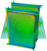
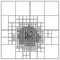
Many of the algorithms of introductory scientific computing have super-linear runtime scaling. Gaussian elimination or LU decomposition are good examples, their runtime scales as $O(n^3)$ with the number of unknowns $n$. Even simple matrix-vector multiplication exhibits quadratic scaling. Problems in scientific computing, especially those arising from science and engineering questions, often demand large-scale computation in order to achieve acceptable fidelity, and such computations will not tolerate super-linear, let alone quadratic or cubic scaling.
This class will teach you a set of techniques and ideas that successfully reduce this asymptotic cost for an important set of operations. This leads to these techniques being called "fast algorithms". We will begin by examining some of these ideas from a linear-algebraic perspective, where for matrices with special structure, large cost gains can be achieved. We will then specialize to PDE boundary value problems, which give rise to many of the largest-scale computations. We will see that integral equations are the natural generalization of the linear-algebraic tools encountered earlier, and we will understand the mathematical and algorithmic foundations that make them powerful tools for computation. All throughout, we will pay much attention to the idea of representation–i.e. the choice of what the numerical unknowns of the system to be solved should be.
Instructor

Course Outline
Note: the section headings in this tree are clickable to reveal more detail.
- Introduction
-
Dense Matrices and Computation
-
Demo: Conditioning of Derivative Matrices
<li data-jstree='{"icon": "fa fa-keyboard-o"}'> <a href="https://mybinder.org/v2/gh/illinois-scicomp/cs598apk-f19-binder/master?filepath=dense_compute/Conditioning of Derivative Matrices.ipynb">Run interactively (on mybinder.org)</a> </li> <li data-jstree='{"icon": "fa fa-terminal"}'> <a href="repocur:demos/upload/dense_compute/Conditioning of Derivative Matrices.py">Download Python script</a> </li> <li data-jstree='{"icon": "fa fa-download"}'> <a href="repocur:demos/upload/dense_compute/Conditioning of Derivative Matrices.ipynb">Download Jupyter notebook</a> </li> </ul> </li> <li data-jstree='{"icon": "fa fa-keyboard-o"}'> <a href="https://mybinder.org/v2/gh/illinois-scicomp/cs598apk-f19-binder/master?filepath=dense_compute/Floating point vs Finite Differences.ipynb">Demo: Floating point vs Finite Differences</a> <ul> <li data-jstree='{"icon": "fa fa-newspaper-o"}'> <a href="repocur:demos/upload/dense_compute/Floating point vs Finite Differences.html">View on the web</a> </li> <li data-jstree='{"icon": "fa fa-keyboard-o"}'> <a href="https://mybinder.org/v2/gh/illinois-scicomp/cs598apk-f19-binder/master?filepath=dense_compute/Floating point vs Finite Differences.ipynb">Run interactively (on mybinder.org)</a> </li> <li data-jstree='{"icon": "fa fa-terminal"}'> <a href="repocur:demos/upload/dense_compute/Floating point vs Finite Differences.py">Download Python script</a> </li> <li data-jstree='{"icon": "fa fa-download"}'> <a href="repocur:demos/upload/dense_compute/Floating point vs Finite Differences.ipynb">Download Jupyter notebook</a> </li> </ul> </li> <li data-jstree='{"icon": "fa fa-keyboard-o"}'> <a href="https://mybinder.org/v2/gh/illinois-scicomp/cs598apk-f19-binder/master?filepath=dense_compute/Rank of a Potential Evaluation Matrix.ipynb">Demo: Rank of a Potential Evaluation Matrix</a> <ul> <li data-jstree='{"icon": "fa fa-newspaper-o"}'> <a href="repocur:demos/upload/dense_compute/Rank of a Potential Evaluation Matrix.html">View on the web</a> </li> <li data-jstree='{"icon": "fa fa-keyboard-o"}'> <a href="https://mybinder.org/v2/gh/illinois-scicomp/cs598apk-f19-binder/master?filepath=dense_compute/Rank of a Potential Evaluation Matrix.ipynb">Run interactively (on mybinder.org)</a> </li> <li data-jstree='{"icon": "fa fa-terminal"}'> <a href="repocur:demos/upload/dense_compute/Rank of a Potential Evaluation Matrix.py">Download Python script</a> </li> <li data-jstree='{"icon": "fa fa-download"}'> <a href="repocur:demos/upload/dense_compute/Rank of a Potential Evaluation Matrix.ipynb">Download Jupyter notebook</a> </li> </ul> </li> </ul> -
Tools for Low-Rank Linear Algebra
- Low-Rank Approximation: Basics
<li data-jstree='{"icon": "fa fa-file-o"}'> Low-Rank Approximation: Error Control </li> <li data-jstree='{"icon": "fa fa-file-o"}'> Reducing Complexity </li> <li data-jstree='{"icon": "fa fa-keyboard-o"}'> <a href="https://mybinder.org/v2/gh/illinois-scicomp/cs598apk-f19-binder/master?filepath=low_rank/Interpolative Decomposition.ipynb">Demo: Interpolative Decomposition</a> <ul> <li data-jstree='{"icon": "fa fa-newspaper-o"}'> <a href="repocur:demos/upload/low_rank/Interpolative Decomposition.html">View on the web</a> </li> <li data-jstree='{"icon": "fa fa-keyboard-o"}'> <a href="https://mybinder.org/v2/gh/illinois-scicomp/cs598apk-f19-binder/master?filepath=low_rank/Interpolative Decomposition.ipynb">Run interactively (on mybinder.org)</a> </li> <li data-jstree='{"icon": "fa fa-terminal"}'> <a href="repocur:demos/upload/low_rank/Interpolative Decomposition.py">Download Python script</a> </li> <li data-jstree='{"icon": "fa fa-download"}'> <a href="repocur:demos/upload/low_rank/Interpolative Decomposition.ipynb">Download Jupyter notebook</a> </li> </ul> </li> <li data-jstree='{"icon": "fa fa-keyboard-o"}'> <a href="https://mybinder.org/v2/gh/illinois-scicomp/cs598apk-f19-binder/master?filepath=low_rank/Randomized SVD.ipynb">Demo: Randomized SVD</a> <ul> <li data-jstree='{"icon": "fa fa-newspaper-o"}'> <a href="repocur:demos/upload/low_rank/Randomized SVD.html">View on the web</a> </li> <li data-jstree='{"icon": "fa fa-keyboard-o"}'> <a href="https://mybinder.org/v2/gh/illinois-scicomp/cs598apk-f19-binder/master?filepath=low_rank/Randomized SVD.ipynb">Run interactively (on mybinder.org)</a> </li> <li data-jstree='{"icon": "fa fa-terminal"}'> <a href="repocur:demos/upload/low_rank/Randomized SVD.py">Download Python script</a> </li> <li data-jstree='{"icon": "fa fa-download"}'> <a href="repocur:demos/upload/low_rank/Randomized SVD.ipynb">Download Jupyter notebook</a> </li> </ul> </li> <li data-jstree='{"icon": "fa fa-keyboard-o"}'> <a href="https://mybinder.org/v2/gh/illinois-scicomp/cs598apk-f19-binder/master?filepath=low_rank/Rank-Revealing QR.ipynb">Demo: Rank-Revealing QR</a> <ul> <li data-jstree='{"icon": "fa fa-newspaper-o"}'> <a href="repocur:demos/upload/low_rank/Rank-Revealing QR.html">View on the web</a> </li> <li data-jstree='{"icon": "fa fa-keyboard-o"}'> <a href="https://mybinder.org/v2/gh/illinois-scicomp/cs598apk-f19-binder/master?filepath=low_rank/Rank-Revealing QR.ipynb">Run interactively (on mybinder.org)</a> </li> <li data-jstree='{"icon": "fa fa-terminal"}'> <a href="repocur:demos/upload/low_rank/Rank-Revealing QR.py">Download Python script</a> </li> <li data-jstree='{"icon": "fa fa-download"}'> <a href="repocur:demos/upload/low_rank/Rank-Revealing QR.ipynb">Download Jupyter notebook</a> </li> </ul> </li> </ul> -
Rank and Smoothness
- Local Expansions
<li data-jstree='{"icon": "fa fa-file-o"}'> Multipole Expansions </li> <li data-jstree='{"icon": "fa fa-file-o"}'> Rank Estimates </li> <li data-jstree='{"icon": "fa fa-file-o"}'> Proxy Expansions </li> <li data-jstree='{"icon": "fa fa-keyboard-o"}'> <a href="https://mybinder.org/v2/gh/illinois-scicomp/cs598apk-f19-binder/master?filepath=rank_smoothness/Checking Rank Estimates.ipynb">Demo: Checking Rank Estimates</a> <ul> <li data-jstree='{"icon": "fa fa-newspaper-o"}'> <a href="repocur:demos/upload/rank_smoothness/Checking Rank Estimates.html">View on the web</a> </li> <li data-jstree='{"icon": "fa fa-keyboard-o"}'> <a href="https://mybinder.org/v2/gh/illinois-scicomp/cs598apk-f19-binder/master?filepath=rank_smoothness/Checking Rank Estimates.ipynb">Run interactively (on mybinder.org)</a> </li> <li data-jstree='{"icon": "fa fa-terminal"}'> <a href="repocur:demos/upload/rank_smoothness/Checking Rank Estimates.py">Download Python script</a> </li> <li data-jstree='{"icon": "fa fa-download"}'> <a href="repocur:demos/upload/rank_smoothness/Checking Rank Estimates.ipynb">Download Jupyter notebook</a> </li> </ul> </li> <li data-jstree='{"icon": "fa fa-keyboard-o"}'> <a href="https://mybinder.org/v2/gh/illinois-scicomp/cs598apk-f19-binder/master?filepath=rank_smoothness/Multipole and Local Expansions.ipynb">Demo: Multipole and Local Expansions</a> <ul> <li data-jstree='{"icon": "fa fa-newspaper-o"}'> <a href="repocur:demos/upload/rank_smoothness/Multipole and Local Expansions.html">View on the web</a> </li> <li data-jstree='{"icon": "fa fa-keyboard-o"}'> <a href="https://mybinder.org/v2/gh/illinois-scicomp/cs598apk-f19-binder/master?filepath=rank_smoothness/Multipole and Local Expansions.ipynb">Run interactively (on mybinder.org)</a> </li> <li data-jstree='{"icon": "fa fa-terminal"}'> <a href="repocur:demos/upload/rank_smoothness/Multipole and Local Expansions.py">Download Python script</a> </li> <li data-jstree='{"icon": "fa fa-download"}'> <a href="repocur:demos/upload/rank_smoothness/Multipole and Local Expansions.ipynb">Download Jupyter notebook</a> </li> </ul> </li> <li data-jstree='{"icon": "fa fa-keyboard-o"}'> <a href="https://mybinder.org/v2/gh/illinois-scicomp/cs598apk-f19-binder/master?filepath=rank_smoothness/Skeletonization using Proxies.ipynb">Demo: Skeletonization using Proxies</a> <ul> <li data-jstree='{"icon": "fa fa-newspaper-o"}'> <a href="repocur:demos/upload/rank_smoothness/Skeletonization using Proxies.html">View on the web</a> </li> <li data-jstree='{"icon": "fa fa-keyboard-o"}'> <a href="https://mybinder.org/v2/gh/illinois-scicomp/cs598apk-f19-binder/master?filepath=rank_smoothness/Skeletonization using Proxies.ipynb">Run interactively (on mybinder.org)</a> </li> <li data-jstree='{"icon": "fa fa-terminal"}'> <a href="repocur:demos/upload/rank_smoothness/Skeletonization using Proxies.py">Download Python script</a> </li> <li data-jstree='{"icon": "fa fa-download"}'> <a href="repocur:demos/upload/rank_smoothness/Skeletonization using Proxies.ipynb">Download Jupyter notebook</a> </li> </ul> </li> </ul> -
Near and Far: Separating out High-Rank Interactions
- Ewald Summation
<li data-jstree='{"icon": "fa fa-file-o"}'> Barnes-Hut </li> <li data-jstree='{"icon": "fa fa-file-o"}'> Fast Mutipole </li> <li data-jstree='{"icon": "fa fa-file-o"}'> Direct Solvers </li> <li data-jstree='{"icon": "fa fa-file-o"}'> The Butterfly Factorization </li> <li data-jstree='{"icon": "fa fa-keyboard-o"}'> <a href="https://mybinder.org/v2/gh/illinois-scicomp/cs598apk-f19-binder/master?filepath=near_and_far/Butterfly Factorization.ipynb">Demo: Butterfly Factorization</a> <ul> <li data-jstree='{"icon": "fa fa-newspaper-o"}'> <a href="repocur:demos/upload/near_and_far/Butterfly Factorization.html">View on the web</a> </li> <li data-jstree='{"icon": "fa fa-keyboard-o"}'> <a href="https://mybinder.org/v2/gh/illinois-scicomp/cs598apk-f19-binder/master?filepath=near_and_far/Butterfly Factorization.ipynb">Run interactively (on mybinder.org)</a> </li> <li data-jstree='{"icon": "fa fa-terminal"}'> <a href="repocur:demos/upload/near_and_far/Butterfly Factorization.py">Download Python script</a> </li> <li data-jstree='{"icon": "fa fa-download"}'> <a href="repocur:demos/upload/near_and_far/Butterfly Factorization.ipynb">Download Jupyter notebook</a> </li> </ul> </li> </ul> - Outlook: Building a Fast PDE Solver
-
Going Infinite: Integral Operators and Functional Analysis
- Norms and Operators
<li data-jstree='{"icon": "fa fa-file-o"}'> Compactness </li> <li data-jstree='{"icon": "fa fa-file-o"}'> Integral Operators </li> <li data-jstree='{"icon": "fa fa-file-o"}'> Riesz and Fredholm </li> <li data-jstree='{"icon": "fa fa-file-o"}'> A Tiny Bit of Spectral Theory </li> </ul> -
Singular Integrals and Potential Theory
- Singular Integrals
<li data-jstree='{"icon": "fa fa-file-o"}'> Green's Formula and Its Consequences </li> <li data-jstree='{"icon": "fa fa-file-o"}'> Jump Relations </li> </ul> -
Boundary Value Problems
- Laplace
<li data-jstree='{"icon": "fa fa-file-o"}'> Helmholtz </li> <li data-jstree='{"icon": "fa fa-file-o"}'> Calderón identities </li> </ul> -
Back from Infinity: Discretization
- Fundamentals: Meshes, Functions, and Approximation
<li data-jstree='{"icon": "fa fa-file-o"}'> Integral Equation Discretizations </li> <li data-jstree='{"icon": "fa fa-file-o"}'> Integral Equation Discretizations: Nyström </li> <li data-jstree='{"icon": "fa fa-file-o"}'> Integral Equation Discretizations: Projection </li> <li data-jstree='{"icon": "fa fa-keyboard-o"}'> <a href="https://mybinder.org/v2/gh/illinois-scicomp/cs598apk-f19-binder/master?filepath=discretization/2D Interpolation Nodes.ipynb">Demo: 2D Interpolation Nodes</a> <ul> <li data-jstree='{"icon": "fa fa-newspaper-o"}'> <a href="repocur:demos/upload/discretization/2D Interpolation Nodes.html">View on the web</a> </li> <li data-jstree='{"icon": "fa fa-keyboard-o"}'> <a href="https://mybinder.org/v2/gh/illinois-scicomp/cs598apk-f19-binder/master?filepath=discretization/2D Interpolation Nodes.ipynb">Run interactively (on mybinder.org)</a> </li> <li data-jstree='{"icon": "fa fa-terminal"}'> <a href="repocur:demos/upload/discretization/2D Interpolation Nodes.py">Download Python script</a> </li> <li data-jstree='{"icon": "fa fa-download"}'> <a href="repocur:demos/upload/discretization/2D Interpolation Nodes.ipynb">Download Jupyter notebook</a> </li> </ul> </li> <li data-jstree='{"icon": "fa fa-keyboard-o"}'> <a href="https://mybinder.org/v2/gh/illinois-scicomp/cs598apk-f19-binder/master?filepath=discretization/Choice of Nodes for Polynomial Interpolation.ipynb">Demo: Choice of Nodes for Polynomial Interpolation</a> <ul> <li data-jstree='{"icon": "fa fa-newspaper-o"}'> <a href="repocur:demos/upload/discretization/Choice of Nodes for Polynomial Interpolation.html">View on the web</a> </li> <li data-jstree='{"icon": "fa fa-keyboard-o"}'> <a href="https://mybinder.org/v2/gh/illinois-scicomp/cs598apk-f19-binder/master?filepath=discretization/Choice of Nodes for Polynomial Interpolation.ipynb">Run interactively (on mybinder.org)</a> </li> <li data-jstree='{"icon": "fa fa-terminal"}'> <a href="repocur:demos/upload/discretization/Choice of Nodes for Polynomial Interpolation.py">Download Python script</a> </li> <li data-jstree='{"icon": "fa fa-download"}'> <a href="repocur:demos/upload/discretization/Choice of Nodes for Polynomial Interpolation.ipynb">Download Jupyter notebook</a> </li> </ul> </li> <li data-jstree='{"icon": "fa fa-keyboard-o"}'> <a href="https://mybinder.org/v2/gh/illinois-scicomp/cs598apk-f19-binder/master?filepath=discretization/Vandermonde conditioning.ipynb">Demo: Vandermonde conditioning</a> <ul> <li data-jstree='{"icon": "fa fa-newspaper-o"}'> <a href="repocur:demos/upload/discretization/Vandermonde conditioning.html">View on the web</a> </li> <li data-jstree='{"icon": "fa fa-keyboard-o"}'> <a href="https://mybinder.org/v2/gh/illinois-scicomp/cs598apk-f19-binder/master?filepath=discretization/Vandermonde conditioning.ipynb">Run interactively (on mybinder.org)</a> </li> <li data-jstree='{"icon": "fa fa-terminal"}'> <a href="repocur:demos/upload/discretization/Vandermonde conditioning.py">Download Python script</a> </li> <li data-jstree='{"icon": "fa fa-download"}'> <a href="repocur:demos/upload/discretization/Vandermonde conditioning.ipynb">Download Jupyter notebook</a> </li> </ul> </li> <li data-jstree='{"icon": "fa fa-keyboard-o"}'> <a href="https://mybinder.org/v2/gh/illinois-scicomp/cs598apk-f19-binder/master?filepath=discretization/Visualizing the 2D PKDO Basis.ipynb">Demo: Visualizing the 2D PKDO Basis</a> <ul> <li data-jstree='{"icon": "fa fa-newspaper-o"}'> <a href="repocur:demos/upload/discretization/Visualizing the 2D PKDO Basis.html">View on the web</a> </li> <li data-jstree='{"icon": "fa fa-keyboard-o"}'> <a href="https://mybinder.org/v2/gh/illinois-scicomp/cs598apk-f19-binder/master?filepath=discretization/Visualizing the 2D PKDO Basis.ipynb">Run interactively (on mybinder.org)</a> </li> <li data-jstree='{"icon": "fa fa-terminal"}'> <a href="repocur:demos/upload/discretization/Visualizing the 2D PKDO Basis.py">Download Python script</a> </li> <li data-jstree='{"icon": "fa fa-download"}'> <a href="repocur:demos/upload/discretization/Visualizing the 2D PKDO Basis.ipynb">Download Jupyter notebook</a> </li> </ul> </li> <li data-jstree='{"icon": "fa fa-keyboard-o"}'> <a href="https://mybinder.org/v2/gh/illinois-scicomp/cs598apk-f19-binder/master?filepath=discretization/Working with Unstructured Meshes.ipynb">Demo: Working with Unstructured Meshes</a> <ul> <li data-jstree='{"icon": "fa fa-newspaper-o"}'> <a href="repocur:demos/upload/discretization/Working with Unstructured Meshes.html">View on the web</a> </li> <li data-jstree='{"icon": "fa fa-keyboard-o"}'> <a href="https://mybinder.org/v2/gh/illinois-scicomp/cs598apk-f19-binder/master?filepath=discretization/Working with Unstructured Meshes.ipynb">Run interactively (on mybinder.org)</a> </li> <li data-jstree='{"icon": "fa fa-terminal"}'> <a href="repocur:demos/upload/discretization/Working with Unstructured Meshes.py">Download Python script</a> </li> <li data-jstree='{"icon": "fa fa-download"}'> <a href="repocur:demos/upload/discretization/Working with Unstructured Meshes.ipynb">Download Jupyter notebook</a> </li> </ul> </li> </ul> -
Computing Integrals: Approaches to Quadrature
- A Bag of Quadrature Tricks
<li data-jstree='{"icon": "fa fa-file-o"}'> Quadrature by expansion (`QBX') </li> <li data-jstree='{"icon": "fa fa-file-o"}'> QBX Acceleration </li> <li data-jstree='{"icon": "fa fa-file-o"}'> Reducing Complexity through better Expansions </li> <li data-jstree='{"icon": "fa fa-file-o"}'> Results: Layer Potentials </li> <li data-jstree='{"icon": "fa fa-file-o"}'> Results: Poisson </li> <li data-jstree='{"icon": "fa fa-keyboard-o"}'> <a href="https://mybinder.org/v2/gh/illinois-scicomp/cs598apk-f19-binder/master?filepath=quadrature/Kussmaul-Martensen quadrature.ipynb">Demo: Kussmaul-Martensen quadrature</a> <ul> <li data-jstree='{"icon": "fa fa-newspaper-o"}'> <a href="repocur:demos/upload/quadrature/Kussmaul-Martensen quadrature.html">View on the web</a> </li> <li data-jstree='{"icon": "fa fa-keyboard-o"}'> <a href="https://mybinder.org/v2/gh/illinois-scicomp/cs598apk-f19-binder/master?filepath=quadrature/Kussmaul-Martensen quadrature.ipynb">Run interactively (on mybinder.org)</a> </li> <li data-jstree='{"icon": "fa fa-terminal"}'> <a href="repocur:demos/upload/quadrature/Kussmaul-Martensen quadrature.py">Download Python script</a> </li> <li data-jstree='{"icon": "fa fa-download"}'> <a href="repocur:demos/upload/quadrature/Kussmaul-Martensen quadrature.ipynb">Download Jupyter notebook</a> </li> </ul> </li> </ul> - Going General: More PDEs
-
Demo: Conditioning of Derivative Matrices
CAUTION!
These scribbled PDFs are an unedited reflection of what we wrote during class. They need to be viewed in the context of the class discussion that led to them. See the lecture videos for that.
If you would like actual, self-contained class notes, look in the outline above.
These scribbles are provided here to provide a record of our class discussion, to be used in perhaps the following ways:
- as a way to cross-check your own notes
- to look up a formula that you know was shown in a certain class
- to remind yourself of what exactly was covered on a given day
By continuing to read them, you acknowledge that these files are provided as supplementary material on an as-is basis.
- scribbles-2019-08-28.pdf
- scribbles-2019-08-30.pdf
- scribbles-2019-09-04.pdf
- scribbles-2019-09-06.pdf
- scribbles-2019-09-11.pdf
- scribbles-2019-09-13.pdf
- scribbles-2019-09-18.pdf
- scribbles-2019-09-20.pdf
- scribbles-2019-09-25.pdf
- scribbles-2019-09-27.pdf
- scribbles-2019-10-02.pdf
- scribbles-2019-10-09.pdf
- scribbles-2019-10-11.pdf
- scribbles-2019-10-16.pdf
- scribbles-2019-10-18.pdf
- scribbles-2019-10-23.pdf
- scribbles-2019-10-25.pdf
- scribbles-2019-10-30.pdf
- scribbles-2019-11-01.pdf
- scribbles-2019-11-06.pdf
- scribbles-2019-11-08.pdf
- scribbles-2019-11-13.pdf
- scribbles-2019-11-15.pdf
- scribbles-2019-11-20.pdf
- scribbles-2019-11-22.pdf
Computing
We will be using Python with the libraries numpy, scipy and matplotlib for assignments. No other languages are permitted. Python has a very gentle learning curve, so you should feel at home even if you've never done any work in Python.
Virtual Machine Image
While you are free to install Python and Numpy on your own computer to do homework, the only supported way to do so is using the supplied virtual machine image.
Books and Papers
Randomized Linear Algebra
Fast Multipole
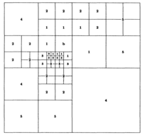
Carrier, Greengard, Rokhlin: A Fast Adaptive Multipole Algorithm for Particle Simulations
Further references:
- A fast algorithm for particle simulations by Greengard and Rokhlin.
Integral Equations/Functional Analysis
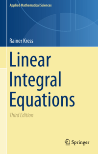
Rainer Kress, Linear integral equations. (second edition) The references in the notes are for the second edition.
A third edition is also available.
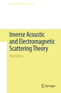
David Colton and Rainer Kress, Inverse Acoustic and Electromagnetic Scattering Theory. (3rd edition)
Background: Numerical Linear Algebra
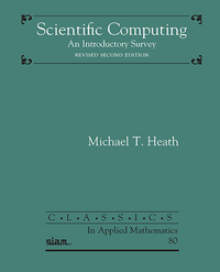
Scientific Computing: An Introductory Survey / E-Book (accessible free of charge from campus network/VPN)
Michael T. Heath, Revised Second Edition, Society for Industrial and Applied Mathematics
Further references:
-
Golub and van Loan is the definitive reference, with an emphasis on reference
-
Trefethen and Bau is less comprehensive but more approachable
Previous editions of this class
Related Classes Elsewhere
- Alex Barnett (Dartmouth)
- Shravan Veerapaneni (Michigan)
- Leslie Greengard (NYU)
- Gunnar Martinsson: UC Boulder Dartmouth
- Jianlin Xia (Purdue)
- Francesco Andriulli (ENS TELECOM Bretagne)
- Mark Tygert
Python Help
- Python tutorial
- Facts and myths about Python names and values
- Dive into Python 3
- Learn Python the hard way
- Project Euler (Lots of practice problems)
Numpy Help
- Introduction to Python for Science
- The SciPy lectures
- The Numpy MedKit by Stéfan van der Walt
- The Numpy User Guide by Travis Oliphant
- Numpy/Scipy documentation
- More in this reddit thread
- Spyder (a Python IDE, like Matlab) is installed in the virtual machine. (Applications Menu > Development > Spyder)
- An introduction to Numpy and SciPy
- 100 Numpy exercises